
author
What is AWS Data Wrangler library ? The GitHub page of the project describes the library as Pandas on AWS.
In case, you stayed in your cave for a long time, Pandas is an open source data analysis and manipulation tool, built on top of the Python programming language. Pandas is designed to be fast, powerful, flexible and easy to use.
Positioning itself a “ Pandas on AWS ” immediately raises the bar.
It is a project available from the GitHub organization AWSLab. You can find the organization page a bunch of projects open sourced by AWS, some of them more or less used or mature. The s2n project, an implementation of the TLS/SSL protocols, is a good example of mature projects available.
AWS Data Wrangler module represents to date, more than 771 commits, 20 contributors, and 52 releases. Versions are currently released at a sustained pace, and the Python module is currently available in version 1.4.0.
Installation
There are two ways to install the module. Either using pip or using Conda.
Pip install
To install the module with pip, you can use the following command:
pip install awswrangler
Conda install
If you are a Conda user, instead, you can install the module with the following command:
conda install -c conda-forge awswrangler
Basic usage
Following the GitHub readme introduction, here is the way to create a basic DataFrame with Pandas:
import pandas as pd

df = pd.DataFrame({"id": [1, 2], "value": ["foo", "bar"]})
And, then import the AWS Data Wrangler module:
import awswrangler as wr
Write data to Amazon S3
Now, lets create, into an S3 bucket, a data file representing the data from the DataFrame serialized into a file:
# Storing data on Data Lake
wr.s3.to_parquet(
    df=df,
    path="s3://bucket/dataset/",
    dataset=True,
    database="my_db",
    table="my_table"
)
Easy ! An s3 variable at the root of the AWS Data Wrangler module lets the user access functions allowing to interact with s3, in this case to flush the DataFrame to S3.
Read data from Amazon S3
The reverse function is also available allowing to read the data from S3:
# Retrieving the data directly from Amazon S3
df = wr.s3.read_parquet("s3://bucket/dataset/", dataset=True)
You may wonder what is possible to do with the AWS Data Wrangler package apart interacting with S3. Let's take a free tour over some of the libraries features to discover some of its capabilities.
Definition
Here is an accurate definition of the library as displayed in the documentation:
An open-source Python package that extends the power of Pandas library to AWS connecting DataFrames and AWS data related services (Amazon Redshift, AWS Glue, Amazon Athena, Amazon EMR, etc).
Built on top of other open-source projects like Pandas, Apache Arrow, Boto3, s3fs, SQLAlchemy, Psycopg2 and PyMySQL, it offers abstracted functions to execute usual ETL tasks like load/unload data from Data Lakes, Data Warehouses and Databases.
Supported services
The aim of the library is to simplify interaction with the data across AWS supported services. Basically, AWS Data Wrangler library is supporting 5 services from AWS:
- Amazon S3
- AWS Glue Catalog
- Amazon Athena
- Databases (Redshift, PostgreSQL & Mysql)
- EMR
- CloudWatch Logs
As the library extends the power of Pandas library to AWS connecting DataFrames and AWS data related services, most of operations available, directly dealing with loading or flushing the data, will rely on Pandas DataFrames.
Simplifying interactions
However, the package is not focused only on loading / unloading the data. The package is also meant to simplify things, more specifically, simplifying interactions with services.
The library provides, for example, functions to :
- Load / unload data for Redshift
- Generate a Redshift copy manifest instead of having to generate it by yourself
but also to :
- simplify create of EMR clusters or definition and submission of build steps.
Interacting with AWS Athena
Interacting with AWS Athena can be cumbersome. To reduce the burden, you have access to functions making things easier, for example, to start, stop, or wait for query completion.
Goodness does not stop on AWS Athena simplified interactions. You will also find improvements in interacting with AWS Glue Data Catalog, making code writing straightforward.
AWS Data Wrangler as default way to interact ?
Given all this improvements made available over the standard APIs, it should be a no brainer to use it as your default way to interact with the supported services in a data processing context with Python.
Lets now go deeper in more detailed examples and notions around the AWS Data Wrangler package. To do that, let's start with sessions.
Sessions
AWS Data Wrangler interacts with AWS services using a default Boto3 Session. That's why, you won't have to provide most of the time any session informations. However, if you need to customize the session the module is working with, it is possible to reconfigure default boto3 session:
boto3.setup_default_session(region_name="eu-west-1")
or even instantiate a new boto3 session, and passing it as a named parameter to function calls:
session = boto3.Session(region_name="us-east-2")
wr.s3.does_object_exist("s3://foo/bar", boto3_session=session)
Amazon S3
As mentioned previously, an s3 variable is available at the root of the AWS Data Wrangler module. The s3 variable will essentially allow you to interact with Amazon S3 service to work on CSV, JSON, Parquet and fixed-width formatted files along with having access to some handy functions purely related to file manipulations.
Lets define first 2 DataFrames:
import awswrangler as wr
import pandas as pd
import boto3

df1 = pd.DataFrame({
    "id": [1, 2],
    "name": ["foo", "boo"]
})

df2 = pd.DataFrame({
    "id": [3],
    "name": ["bar"]
})
Having those 2 DataFrames created, it will be possible to write them simply to S3 this way:
bucket = "my-bucket"

path1 = f"s3://{bucket}/csv/file1.csv"
path2 = f"s3://{bucket}/csv/file2.csv"

wr.s3.to_csv(df1, path1, index=False)
wr.s3.to_csv(df2, path2, index=False)
As a result, it is also possible to read the previously written files in similar fashion:
df1Bis = wr.s3.read_csv(path1)
df1bis and df1 should present the exact same data.
Finally, it is also possible to re-read written data by reading multiple CSV files at once, listing explicitly which files have to be read:
wr.s3.read_csv([path1, path2])
Things can be made even easier by providing only the prefix to read data from:
wr.s3.read_csv(f"s3://{bucket}/csv/")
As seen, in example before, it is very easy to interact with S3, without having to deal with code complexities or boilerplates.
AWS Glue Data Catalog
Having tried a demo of the library interacting with Amazon S3, the next step is to let the user interact directly with the AWS Glue Data Catalog ?
To interact with, the user just have to use the catalog variable on the module.
wr.catalog.databases()
Previous command should return the database list this way:
| Database | Description | |
|---|---|---|
| 0 | awswrangler_test | AWS Data Wrangler Test Arena - Glue Database |
| 1 | default | Default Hive database |
| 2 | sampledb | Sample database |
It may not be that simple with direct usage of boto3 API. But it will be that simple also to list available tables in a specific Database:
wr.catalog.tables(database="awswrangler_test")
The command should return the following result:
| Database | Table | Description | Columns | Partitions | |
| 0 | awswrangler_test | lambda | col1, col2 | ||
| 1 | awswrangler_test | noaa | id, dt, element, value, m_flag, q_flag, s_flag... |
Now, to get table details, meaning column informations, there is just the need to call the table() function over the catalog variable.
wr.catalog.table(database="awswrangler_test", table="boston")
The command should return the following field list:
| Column Name | Type | Partition | Comment | |
| 0 | crim | double | False | per capita crime rate by town |
| 1 | zn | double | False | proportion of residential land zoned for lots ... |
| 2 | indus | double | False | proportion of non-retail business acres per town |
| 3 | chas | double | False | Charles River dummy variable (= 1 if tract bou... |
| 4 | nox | double | False | nitric oxides concentration (parts per 10 mill... |
| 5 | rm | double | False | average number of rooms per dwelling |
| 6 | age | double | False | proportion of owner-occupied units built prior... |
| 7 | dis | double | False | weighted distances to five Boston employment c... |
| 8 | rad | double | False | index of accessibility to radial highways |
| 9 | tax | double | False | full-value property-tax rate per $10,000 |
| 10 | ptratio | double | False | pupil-teacher ratio by town |
| 11 | b | double | False | 1000(Bk - 0.63)^2 where Bk is the proportion o... |
| 12 | lstat | double | False | lower status of the population |
| 13 | target | double | False |
You may wonder however how to create a table, let's say in Parquet format. To proceed, you have to call the function to_parquet() on s3 variable providing the required parameters:
| Parameter | Type | Description |
|---|---|---|
| df | pandas.DataFrame | Pandas DataFrame https://pandas.pydata.org/pandas-docs/stable/reference/api/pandas.DataFrame.html |
| path | str | S3 path (for file e.g. s3://bucket/prefix/filename.parquet) (for dataset e.g. s3://bucket/prefix) |
| dataset | bool | If True store a parquet dataset instead of a single file. If True, enable all follow arguments: partition_cols, mode, database, table, description, parameters, columns_comments. |
| database | str, optional | Glue/Athena catalog: Database name. |
| table | str, optional | Glue/Athena catalog: Table name |
| mode | str, optional | append (Default), overwrite, overwrite_partitions. Only takes effect if dataset=True |
| description | str, optional | |
| parameters | Dict[str, str], optional | |
| columns_comments | Dict[str, str], optional |
All parameters can be found at the following URL: https://aws-data-wrangler.readthedocs.io/en/latest/stubs/awswrangler.s3.to_parquet.html#awswrangler.s3.to_parquet.
Writing a pandas DataFrame to S3 in Parquet format, and referencing it in Glue Data Catalog, can be done this way with the following code:
desc = """This is a copy of UCI ML housing dataset. https://archive.ics.uci.edu/ml/machine-learning-databases/housing/
This dataset was taken from the StatLib library which is maintained at Carnegie Mellon University.
The Boston house-price data of Harrison, D. and Rubinfeld, D.L. ‘Hedonic prices and the demand for clean air’, J. Environ. Economics & Management, vol.5, 81-102, 1978. Used in Belsley, Kuh & Welsch, ‘Regression diagnostics …’, Wiley, 1980. N.B. Various transformations are used in the table on pages 244-261 of the latter.
The Boston house-price data has been used in many machine learning papers that address regression problems.
"""

param = {
    "source": "scikit-learn",
    "class": "cities"
}

comments = {
    "crim": "per capita crime rate by town",
    "zn": "proportion of residential land zoned for lots over 25,000 sq.ft.",
    "indus": "proportion of non-retail business acres per town",
    "chas": "Charles River dummy variable (= 1 if tract bounds river; 0 otherwise)",
    "nox": "nitric oxides concentration (parts per 10 million)",
    "rm": "average number of rooms per dwelling",
    "age": "proportion of owner-occupied units built prior to 1940",
    "dis": "weighted distances to five Boston employment centres",
    "rad": "index of accessibility to radial highways",
    "tax": "full-value property-tax rate per $10,000",
    "ptratio": "pupil-teacher ratio by town",
    "b": "1000(Bk - 0.63)^2 where Bk is the proportion of blacks by town",
    "lstat": "lower status of the population",
}

res = wr.s3.to_parquet(
    df=df,
    path=f"s3://{bucket}/boston",
    dataset=True,
    database="awswrangler_test",
    table="boston",
    mode="overwrite",
    description=desc,
    parameters=param,
    columns_comments=comments
)
This code example is sourced from the AWS Data Wrangler tutorials, and more specifically the following one: https://github.com/awslabs/aws-data-wrangler/blob/master/tutorials/005%20-%20Glue%20Catalog.ipynb.
The execution of previous code sample in AWS Glue Data Catalog results in the following table informations:
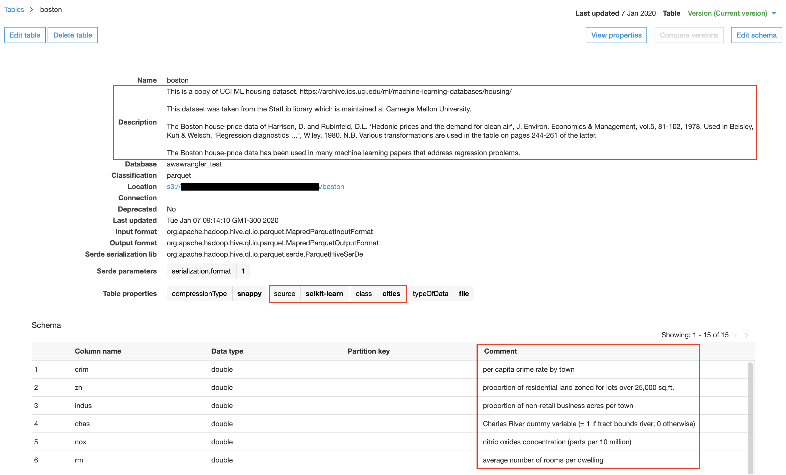
AWS Athena
Now that we have learned to interact with Amazon S3 and AWS Glue Data Catalog, and that we know how to flush DataFrames in S3 and reference it as a dataset in the Data Catalog, we can focus on how to interact with data stored with the service AWS Athena.
AWS Data Wrangler allows to run queries on Athena and fetches results in two ways:
- Using CTAS (ctas_approach=True), which is the default method.
- Using regular queries (ctas_approach=True), and parsing CSV results on S3.
ctas_approach=True
As mentioned in tutorials, this first approach allows to wrap the query with a CTAS, and read the table data as parquet directly from S3. It is faster as it relies on Parquet and not CSV, but it also enables support for nested types. It is mostly a trick compared to the original approach provided officially by the API, but it is effective and fully legal.
The counterpart to use this approach is that you need additional permissions on Glue (Requires create/delete table permissions). The background mechanism is based on the creation of a temporary table that will be immediately deleted after consumption.
Query example:
wr.athena.read_sql_query("SELECT * FROM noaa", database="awswrangler_test")
****ctas_approach=False
Using the regular approach parsing the resulting CSV on S3 provided as query execution result does not requires additional permissions. The read of results will not be as fast as the approach relying on CTAS, but it will anyway be faster than reading results with standard AWS APIs.
Query example:
wr.athena.read_sql_query("SELECT * FROM noaa", database="awswrangler_test", ctas_approach=False)
The only difference with previous example is the change of ctas_approach parameter value from True to False.
Use of categories
Defining DataFrame columns as category allows to optimize the speed of execution, but also helps to save memory. There is only the need to define an additional parameter categories to the function to leverage the improvement.
wr.athena.read_sql_query("SELECT * FROM noaa", database="awswrangler_test", categories=["id", "dt", "element", "value", "m_flag", "q_flag", "s_flag", "obs_time"])
The returned columns are of type pandas.Categorical .
Batching read of results
This option is good for memory constrained environments. Activating this option can be done by passing parameter chunksize. The value provided corresponds to the size of the chunk of data to read. Reading datasets this way allows to limit and constrain memory used, but also implies to read the full results by iterating over chunks.
Query example:
dfs = wr.athena.read_sql_query(
    "SELECT * FROM noaa",
    database="awswrangler_test",
    ctas_approach=False,
    chunksize=10_000_000
)

for df in dfs:  # Batching
    print(len(df.index))
Knowing that big datasets can be challenging to load and read, it is a good workaround to avoid memory issues.
Packaging & Dependencies
Availability as an AWS Lambda layer
Going behind the toy demo, you may wonder how to integrate it with your code. Is it integrable with ease using for example AWS Lambda functions ? Will you have to build a complex pipeline to integrate it the right way into your AWS Lambda package ?
The answer is definitively: No ! A Lambda Layer's zip-file is available along Python wheels & eggs. The Lambda Layers are available at the moment in 3 flavors: Python 3.6, 3.7 & 3.8.
AWS Glue integration
As the AWS Data Wrangler package counts on compiled dependencies (C/C++), there is no support for Glue PySpark by now. Only integration with Glue Python Shell is possible at the moment.
Going one step deeper
If you want to learn more about the library, fee free to read the documentation as it is a good source of inspiration. You can also visit the GitHub repository of the project and crawl the tutorial directory.